

Search Engine Optimization (SEO) often involves combing through large amounts of data when doing research. You might be looking through Google Analytics data for a pattern that can give insight into the best SEO strategy for a website. Or you might be reviewing keyword data to find terms that align with website content. Both of these examples can involve combing through tens of thousands of data points trying to find a handful of nuggets that will give you an idea for your next SEO strategy steps. It is time-consuming, and it can be easy to miss interesting data points in all the noise.
Luckily, Microsoft Excel can do a lot of heavy lifting for you. It can organize and analyze keyword data, such as search volume, competition, and cost per click. Excel can also be used to track on-page SEO metrics, such as title tag length, meta description length, and image alt text. It can audit website crawl errors, identify broken links, and track website loading times. Excel is a powerful tool that can be used to improve your SEO strategy. By learning how to use Excel for SEO, you can save time and improve your results.
Let’s look at how Microsoft Excel can help you understand and review datasets. One of the difficulties when reviewing large amounts of data is that it can become overwhelming. There is superfluous data, text that isn’t in the right format, rows that might be easier to parse if they were in columns, etc. Excel can help you arrange and filter data to make it easier to understand. Here are a few examples.
(Also, if you missed the first part of this series make sure to read Part One here!)
What are Filters in Excel?
Filters are tools in Excel that allow you to temporarily hide or display specific rows of data based on certain criteria. They help you focus on the most relevant information, making it easier to analyze and interpret large datasets. This allows you to quickly isolate and analyze specific information without being overwhelmed by large amounts of information. You can easily spot patterns and trends when you can focus on specific subsets of data. You can also filter different columns to compare and contrast data groups effectively.
Key Features of Filters in Excel:
- Easy to Apply: Simply click the filter button on a column header to access filtering options.
- Versatile Criteria: Filter by text, numbers, dates, or cell formatting.
- Multiple Filters: Apply filters to multiple columns simultaneously for more refined results.
- Custom Filters: Create more complex filtering rules using the “Custom Filter” option.
- Dynamic: Filters only affect the view of the data, not the underlying data itself.
Types of Filters in Excel:
- Text Filters: Filter by specific text values, partial text matches, or conditions like “begins with” or “ends with.”
- Number Filters: Filter by numbers greater than, less than, equal to, or within a certain range.
- Date Filters: Filter by specific dates, date ranges, or conditions like “last month” or “next week.”
- Color Filters: Filter by cell color or font color.
Steps to Apply Filters in Excel:
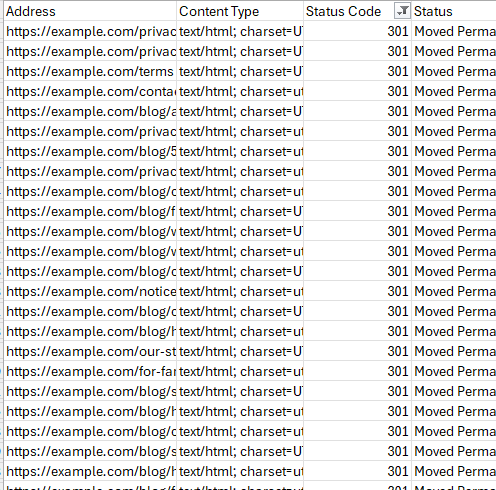
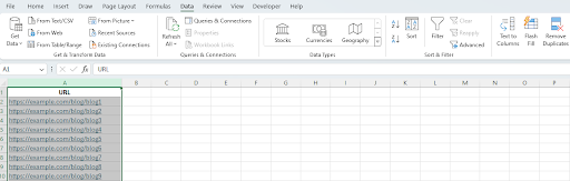
Let’s say you have crawled a site and exported the raw data. You want to isolate all the URLs that are 301 redirects so that you can ensure they are working appropriately. You can use a filter to show only the URLs that have a 301 status code.
Select the column you want to filter (column C in the example below). Click on the Data Tab and then select the filter function.
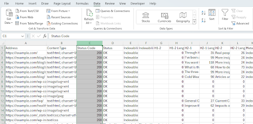
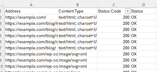
You will now have a filter button at the top of column C:
Click on the filter button. You can use the Select All feature to select and unselect all options. You can also make your selections manually.
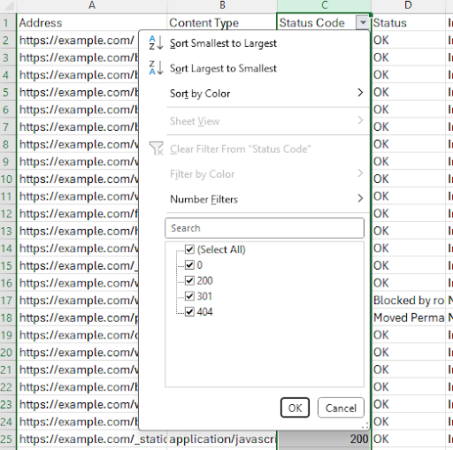
You want to see just the URLs with 301 redirects, so you need to unselect the other options:
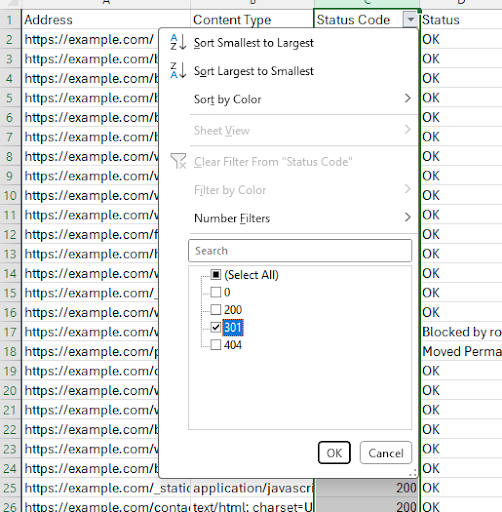
Click OK. You should now see only the URLs with 301s:
Removing Filters:
- To remove filters from a single column: Click the “Clear Filter” button on the column header.
- To remove all filters: Click the “Data” tab and then click the “Clear” button in the “Sort & Filter” section.
Advanced Filters in Excel
- In our example above, we set up a basic filter in Excel. Now let’s talk about Advanced Filters. Advanced filters in Excel go beyond the basic filtering capabilities available through the dropdown menus on column headers. When you’re exploring your data and looking for specific trends or patterns, advanced filters can help you quickly isolate relevant data points based on various conditions. Advanced filters offer a more efficient way to define and apply complex filtering rules when working with large datasets.
Complex Filtering Criteria:
- Multiple conditions: Unlike regular filters where you can only filter by one condition per column, advanced filters allow you to set up multiple criteria for each column you want to filter. This enables you to filter for very specific subsets of data that meet all the defined conditions.
- Logical operators: You can use logical operators like AND, OR, and NOT within your criteria to define complex filtering rules. Imagine you want to find data where a product category is “electronics” AND the price is greater than $100. Advanced filters allow you to set up this kind of multi-layered filtering logic.
Separate Criteria Range:
- Flexibility and Clarity: Advanced filters use a separate criteria range on your spreadsheet to define the filtering conditions. This separates the criteria from the data itself, making your spreadsheet cleaner and easier to manage, especially when dealing with complex filtering rules.
Two Filtering Options:
- Copy to another location: This option allows you to create a filtered copy of your data in a separate location on your spreadsheet. This is useful if you want to keep the original data intact while working with a filtered subset for analysis or presentation.
- Filter the data in-place: This option filters the original data directly, hiding rows that don’t meet the criteria. You can easily toggle the filter on and off to switch between the filtered and complete data view.
How to Use Advanced Filters in Excel:
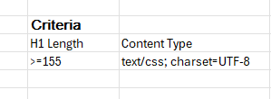
Create a Criteria range. This is an area in the spreadsheet where you define the filter criteria you want. Write the identical column labels as the columns in the dataset you want to filter. Underneath your criteria labels, write the conditions you want to filter for. In the example below, the criteria are that the H1 Length column is equal to or greater than 155 and the Content Type column equals: text/css; charset=UTF-8.
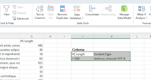
Select your criteria and click on the Advanced option in the Data tab.
A dialog box will appear:
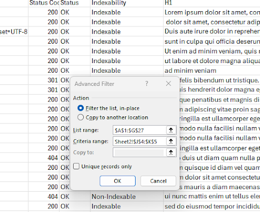
List Range is the range you want to filter. Criteria range is your filter criteria. You can filter the list in-place or copy the results to another location.
The example above filters these results:

This is a simple example, but if you are working with a large amount of data and need to filter for very specific subsets of data, Advanced Filters are extremely valuable. You can add unlimited columns and conditions to your criteria, which allows you to filter for very specific data at a granular level. A list of key options for advanced filters include:
Comparison Operators:
- These operators let you compare data in a column to a specific value or another cell. Common examples include:
- Equal to (=): Filters for rows where the data in that column exactly matches the value you specify.
- Not equal to (<>): Filters for rows where the data in that column is different from the value you specify.
- Greater than (>): Filters for rows where the data in that column is greater than the value you specify.
- Less than (<): Filters for rows where the data in that column is less than the value you specify.
- Greater than or equal to (>=): Filters for rows where the data in that column is greater than or equal to the value you specify.
- Less than or equal to (<=): Filters for rows where the data in that column is less than or equal to the value you specify.
Logical Operators:
- These operators allow you to combine multiple criteria within a single column or across different columns.
- AND: Filters for rows where all specified criteria within a column (connected by AND) must be true. You can use multiple AND statements across different columns to define more complex filters.
- OR: Filters for rows where at least one of the specified criteria within a column (connected by OR) is true.
Text and Wildcard Characters:
- You can filter for text data using wildcards like:
- Asterisk (*): Matches any sequence of characters.
- Question mark (?): Matches any single character.
- For example, “Prod*?” would filter for any product name starting with “Prod” and ending with any single character. Similarly, “col?r” would filter for any color name with four letters where the second letter is unknown.
- Use the tilde (~) before a wildcard character () or (?) to match the literal wildcard character itself. For instance, “~?” would filter for entries containing “?”.
Using Cell References:
- You can reference other cells in your worksheet within your criteria. This allows you to dynamically change the filtering condition based on the value in another cell.
Dates and Numbers:
- You can directly enter dates and numbers as criteria or use Excel functions for more advanced filtering based on date or number comparisons.
Unique Records:
- In the “Advanced Filter” dialog box, you can select the “Unique records only” checkbox to filter your data and only show unique entries.
Why Filters in Excel are an Important Tool for SEO
Overall, filters are essential tools for managing and analyzing data in Excel. With a large spreadsheet, finding specific information can be overwhelming. Filters allow you to quickly narrow down the data to only show rows that meet certain criteria. Filters also make it easier to analyze trends and identify patterns within your data. By filtering based on specific conditions, you can isolate groups of data and see how they compare. They provide an easy and efficient way to focus on the information that matters most, making it easier to extract meaningful insights and make informed decisions. Filters are a powerful tool that can significantly improve your experience working with data in Excel. They make it easier to find information, analyze trends, communicate insights, and manipulate data effectively.
What is Transposing in Excel?
Transposing is the process of flipping the orientation of your data, turning rows into columns, and vice versa. It’s useful for reorganizing data for better analysis, presentation, or compatibility with other programs. It lets you prepare data for charting or graphing that requires data to be in a specific format. It is also useful if you need to copy your data to or from programs that use different data orientations. Transposing helps you create more concise data tables by consolidating multiple rows into fewer columns. There are several ways to apply transposing in Excel.
Methods to Transpose in Excel: Paste Special and Transpose Function
Paste Special:
Select and copy the rows you want to transpose.
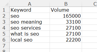
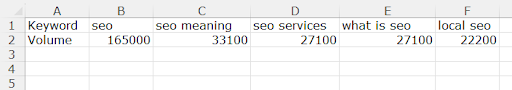
Right-click the first cell in the destination area (where you want the transposed columns to appear). Choose “Paste Special.” Select “Transpose” and click “OK.”
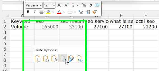
You should now see the original data with the rows and columns transposed:
Additional Tips:
- Create a backup of your data before transposing.
- Ensure the destination area has enough space to accommodate the transposed data.
- Format the transposed data as needed (e.g., adjust column widths, apply cell styles).
Transpose Function:
The TRANSPOSE function in Excel is another way to swap rows and columns of data. The main difference between using PASTE SPECIAL and TRANSPOSE is that the former is static and the latter is dynamic. If your underlying data updates regularly, you may want to use the TRANSPOSE function rather than PASTE SPECIAL.
Here’s a breakdown of how the TRANSPOSE function works:
- Input: The function takes one argument, which is the range of cells you want to transpose.
- Output: The function returns a new range of cells with the rows and columns swapped. For example, if you transpose a range of cells that’s 3 rows tall and 4 columns wide, the output will be a range that’s 4 rows tall and 3 columns wide.
Entering the TRANSPOSE formula:
- Select the destination range: This is where the transposed data will appear. It should have the same number of rows and columns as the original data has columns and rows, respectively.
- Type the formula: In the formula bar, type =TRANSPOSE(.
- Select the range to transpose: Click on the range of cells in your spreadsheet that you want to transpose.
- Close the parenthesis: Type ) after the cell range.
- Enter the formula as an array formula: Since TRANSPOSE is an array formula, you need to press Ctrl+Shift+Enter instead of just Enter to apply the formula. You’ll see curly braces { } appear around the formula to indicate it’s been entered correctly as an array formula. Your results should look like this:
Here are some additional things to keep in mind about the TRANSPOSE function:
- Excel Version: In Excel 365 and Excel 2021 with Dynamic Arrays, the TRANSPOSE function works a bit differently. You can simply enter the formula and press Enter without needing to use Ctrl+Shift+Enter.
Why Transposing Data in Excel is an Important Tool for SEO
Your data might be initially organized for easy input, but analysis might require a different format. Transposing lets you view trends across categories (often in rows) over time (often in columns). This can reveal patterns or relationships that might be hidden in the original format. It is also helpful for formatting charts and graphs, which often need data in a specific orientation. Another way that transposing is useful is if you are merging two datasets and need both to be formatted the same.
Overall, transposing data is a powerful tool in Excel that allows you to manipulate your data to fit your specific needs, ultimately leading to better analysis, clearer presentations, and easier integration with other tools.
What is the Text-to-Columns Function in Excel?
Text-to-columns splits text contained within a single cell into multiple cells, based on specific criteria. An example is splitting the URL slug from the full URL and creating a column just for the slug. Another common use is to split addresses into their basic components. If you have a spreadsheet with complete addresses but you need to filter for a particular state, the text-to-columns feature allows you to split the state into its own column for easy filtering. Text-to-columns is an essential tool for organizing and structuring data for effective analysis and manipulation.
Common Uses:
- Separating full names into first and last names
- Dividing addresses into city, state, and ZIP code
- Splitting product codes into categories and subcategories
- Extracting information from delimited text files (like CSV)
Steps to Use:
- Select the cell(s): Highlight the cells containing the text you want to split.
- Access the Text to Columns wizard: Go to the Data tab and click on Text to Columns.
- Choose a method:
- Delimited: Splits text based on specific characters (e.g., commas, spaces, tabs).
- Fixed width: Splits text at consistent character positions.
- Click the next button.
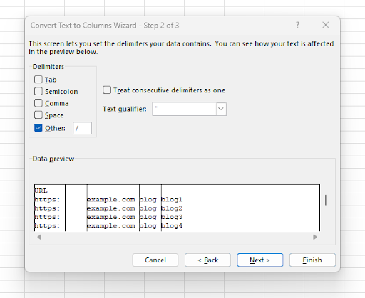
- Set delimiters (if delimited): Select the characters that act as separators in your text.
- The example below shows the delimiters with the / selected as the delimiter. You can use multiple delimiters. Note that the screen gives you a preview of how the text will be split up.
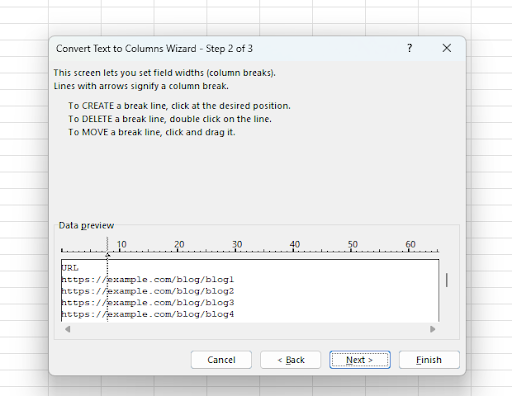
- Set column breaks (if fixed width): Define where each column should start.
- An example of the fixed width screen with the first column break set after the // of the URL.
- Review and adjust format: Use the preview to ensure correct splitting and set the data format for each new column (e.g., text, date).
- Specify destination: Choose where to place the split columns (usually adjacent to the original data).
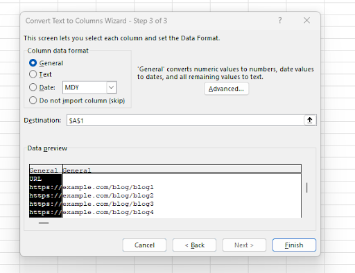
- Finish: Click Finish to apply the changes.
Key Tips:
- Delimiter types: Commas, semicolons, spaces, tabs, custom characters.
- Fixed width: Use the ruler or data preview to accurately set column breaks.
- Data format: Ensure dates, numbers, and text are formatted correctly for analysis.
- Advanced options: Handle complex scenarios like multiple delimiters, consecutive delimiters, and varying widths using advanced settings.
Why Text-to-Columns is an Important Function in Excel
Text-to-columns is a valuable function in Excel because it allows you to transform messy or unformatted data into a structured and usable format. This is particularly important for several reasons. Real-world data often comes from various sources and might not be formatted consistently. Text-to-columns helps you separate data points that are currently combined within a single cell. When data isn’t separated into individual elements, performing calculations or analysis becomes challenging. Text-to-columns helps you structure your data into columns based on specific delimiters (like commas, tabs, spaces), making it easier to apply formulas and functions. This can be crucial for tasks like calculating averages, finding correlations, or creating pivot tables. Many data visualization tools require data to be in a specific format. Text-to-columns plays a key role in preparing your data for creating charts and graphs. In essence, text-to-columns acts as a bridge between raw, unorganized data and meaningful insights. By using it effectively, you can unlock the full potential of your data in Excel, leading to better analysis, clearer presentations, and more informed decision-making.
Excel as an SEO Tool
Even though Excel is not a dedicated SEO platform, it offers important tools for the world of Search Engine Optimization. SEO involves managing a vast amount of data, including keywords, backlinks, competitor analysis results, and website traffic metrics. Excel provides a structured and organized way to store and manage all this information. Extracting insights from SEO data is a valuable method for making informed decisions. Excel offers a variety of formulas and functions to analyze your data to enable you to find meaningful insights. While Excel isn’t a replacement for dedicated SEO tools, it can work seamlessly with them. Many SEO tools allow you to export data in formats compatible with Excel. This lets you import the data into your spreadsheets for further analysis, customization, and integration with your other SEO data. You can create spreadsheets to track keyword rankings, monitor backlinks, analyze competitor strategies, and keep tabs on website traffic trends.
Excel serves as a powerful sidekick for SEO specialists. While it may not be a one-stop shop for all your SEO needs, its data management, analysis, and collaboration capabilities make it a valuable tool for anyone serious about optimizing their website’s search engine ranking. Contact us today to take your SEO to the next level!